
Predicting Diabetes
Classifying Diabetes
Luke Fisher 06 April, 2025
Introduction
Diabetes is an chronic autoimmune disease affecting millions of Americans each year. It is best described as the body’s inability to properly produce insulin, or produce any at all. This is a result of either an invalid or exhausted pancreas, whose job is to secrete enough insulin to manage blood-glucose levels. Normally, insulin is released to enable cells to absorb the blood-glucose to use for energy. In this way, it acts as a “key” between blood-glucose and cells.
For a diabetic, however, this “key” doesn’t occur naturally, instead taking the form of insulin injections. As such, a diabetic uses a glucose monitor to regulate their blood sugar–whose excess or lack thereof has detrimental consequences. For this reason, it is important to know whether or not someone is diabetic. In this project, I will use classification to identify diabetes.
Data Collection
The classification will be based on a dataset from the CDCs Behavioral Risk Factor Surveillance System (BRFSS). The data contains 70,692 responses from the 2015 BRFSS survey, each related to risk factors like smoking, high cholesterol, and physical activity. Furthermore, the data contains an equal 50-50 split of respondents with and without diabetes.
The data is binary, meaning that the predictors take on a value 1 or 0 depending on whether a condition is present. For instance, if a respondent has a smoking habit they will be assigned a 1 for the smoking column; otherwise, they will receive a 0. There are some exceptions to this like BMI and age, where the values are continuous. For our purpose, we will cross-validate the data set.
Methodology
Two classifiers will be built and evaluated using logistic regression and gradient boost. The purpose is to measure their effectiveness in predicting diabetes and select the better model. Both classifiers will predict Diabetes as a binary response variable. The first classifier will start with a logistic model and a function to extract logistic predictions. This function will predict on the logistic model to create labels at multiple cutoffs, taking on the values, respectively, “yes” and “no” for instances of Diabetes above or below a given cutoff. Afterwards, these predicted labels will be compared with the actual values from the data set in a table and put into a confusion matrix for evaluation. The goal is to isolate and optimize one model for classification. Once identified, this model will be further evaluated in its predictive ability with metrics like Accuracy, Sensitivity, Specificity, and ROC-AUC. Additionally, its train and test errors will be included to identify possible under or over-fitting.
The second classifier will use a gradient boost model, xgboost, to predict Diabetes. This model will start with two matrices–one each for the train and test sets–containing the same regression formula as the logistic model. Parameters will then be set up to specify conditions for the boost model, such as learning rate and objective. In this case, the objective of the boost model is to optimize for binary classification through logistic regression. The boost model will be trained on these parameters and predicted on the test matrix. It will be applied to a 0.5 cutoff and evaluated by the same classification metrics as the logistic model, including train and test error. The metrics from the two models will then be evaluated to select the model with the better predictive ability.
library(dplyr)
library(ggplot2)
library(ISLR)
library(tibble)
library(caret)
library(tidyr)
library(skimr)
library(glmnet)
library(car)
library(xgboost)
library(pROC)
library(knitr)
diabetesData <- read.csv('/Users/lukefisher/Desktop/Coding/repos/Health_Analytics/Data/Diabetes_Indicators_Binary.csv')
Data Wrangling
diabetesData <- diabetesData %>%
rename(Diabetes = Diabetes_binary) %>%
mutate(Diabetes = factor(Diabetes, levels = c(0, 1), labels = c("no", "yes")))
# Split the data into an 80/20 train vs. test split. Set the seed for replicability.
set.seed(44222)

diabetesIdx = sample((nrow(diabetesData)), size = 0.8 * nrow(diabetesData))
diabetesTrn = diabetesData[diabetesIdx, ]
diabetesTst = diabetesData[-diabetesIdx, ]

dataHead <- head(diabetesTrn, n = 10)

kable(dataHead)
| Diabetes | HighBP | HighChol | CholCheck | BMI | Smoker | Stroke | HeartDiseaseorAttack | PhysActivity | Fruits | Veggies | HvyAlcoholConsump | AnyHealthcare | NoDocbcCost | GenHlth | MentHlth | PhysHlth | DiffWalk | Sex | Age | Education | Income | |
|---|---|---|---|---|---|---|---|---|---|---|---|---|---|---|---|---|---|---|---|---|---|---|
| 36027 | yes | 0 | 0 | 1 | 32 | 0 | 0 | 0 | 1 | 1 | 1 | 0 | 1 | 0 | 3 | 0 | 0 | 0 | 1 | 11 | 5 | 7 |
| 32605 | no | 1 | 0 | 1 | 29 | 1 | 0 | 1 | 1 | 0 | 1 | 0 | 1 | 0 | 5 | 0 | 28 | 1 | 1 | 9 | 4 | 6 |
| 67519 | yes | 1 | 0 | 1 | 30 | 1 | 1 | 0 | 1 | 0 | 1 | 0 | 1 | 0 | 5 | 0 | 30 | 1 | 1 | 8 | 6 | 7 |
| 41322 | yes | 1 | 0 | 1 | 24 | 1 | 0 | 0 | 1 | 1 | 1 | 0 | 1 | 0 | 2 | 0 | 0 | 0 | 1 | 9 | 4 | 3 |
| 54098 | yes | 1 | 1 | 1 | 28 | 1 | 1 | 1 | 1 | 1 | 1 | 0 | 1 | 0 | 4 | 0 | 0 | 0 | 0 | 13 | 5 | 6 |
| 34711 | no | 0 | 0 | 1 | 26 | 1 | 0 | 0 | 1 | 1 | 1 | 0 | 0 | 0 | 3 | 0 | 0 | 0 | 0 | 3 | 4 | 3 |
| 27963 | no | 0 | 0 | 1 | 36 | 1 | 0 | 0 | 1 | 0 | 1 | 0 | 1 | 0 | 3 | 0 | 2 | 0 | 1 | 6 | 5 | 8 |
| 12132 | no | 0 | 0 | 1 | 28 | 1 | 0 | 0 | 1 | 1 | 1 | 0 | 1 | 0 | 2 | 0 | 0 | 1 | 0 | 8 | 5 | 4 |
| 11078 | no | 0 | 0 | 0 | 22 | 0 | 0 | 0 | 1 | 1 | 1 | 0 | 0 | 1 | 1 | 0 | 0 | 0 | 1 | 6 | 4 | 3 |
| 38966 | yes | 1 | 0 | 1 | 44 | 0 | 0 | 0 | 1 | 1 | 1 | 0 | 1 | 0 | 3 | 2 | 1 | 1 | 0 | 8 | 3 | 3 |
Creating logistic models
get_logistic_pred = function(mod, data, res = "y", pos = 1, neg = 0, cut = 0.5) {
  probs = predict(mod, newdata = data, type = "response")
  ifelse(probs > cut, pos, neg)
}

# Creating separate predictions based on different cutoffs

lrgModel = glm(Diabetes ~ ., data = diabetesTrn, family = "binomial")

testPred_01 = get_logistic_pred(lrgModel, diabetesTst, res = "Diabetes",
pos = "yes", neg = "no", cut = 0.1)

testPred_02 = get_logistic_pred(lrgModel, diabetesTst, res = "Diabetes",
pos = "yes", neg = "no", cut = 0.33)

testPred_03 = get_logistic_pred(lrgModel, diabetesTst, res = "Diabetes",
pos = "yes", neg = "no", cut = 0.5)

testPred_04 = get_logistic_pred(lrgModel, diabetesTst, res = "Diabetes",
pos = "yes", neg = "no", cut = 0.66)

testPred_05 = get_logistic_pred(lrgModel, diabetesTst, res = "Diabetes",
pos = "yes", neg = "no", cut = 0.9)


# Evaluate Accuaracy, Sensitivity, and Specificity for each cutoff
testTab_01 <- table(predicted = testPred_01, actual = diabetesTst$Diabetes)
testTab_02 <- table(predicted = testPred_02, actual = diabetesTst$Diabetes)
testTab_03 <- table(predicted = testPred_03, actual = diabetesTst$Diabetes)
testTab_04 <- table(predicted = testPred_04, actual = diabetesTst$Diabetes)
testTab_05 <- table(predicted = testPred_05, actual = diabetesTst$Diabetes)


testMatrx_01 <- confusionMatrix(testTab_01, positive = "yes")
testMatrx_02 <- confusionMatrix(testTab_02, positive = "yes")
testMatrx_03 <- confusionMatrix(testTab_03, positive = "yes")
testMatrx_04 <- confusionMatrix(testTab_04, positive = "yes")
testMatrx_05 <- confusionMatrix(testTab_05, positive = "yes")


metrics <- rbind(
  c(testMatrx_01$overall["Accuracy"],
    testMatrx_01$byClass["Sensitivity"],
    testMatrx_01$byClass["Specificity"]),

  c(testMatrx_02$overall["Accuracy"],
    testMatrx_02$byClass["Sensitivity"],
    testMatrx_02$byClass["Specificity"]),

  c(testMatrx_03$overall["Accuracy"],
    testMatrx_03$byClass["Sensitivity"],
    testMatrx_03$byClass["Specificity"]),

  c(testMatrx_04$overall["Accuracy"],
    testMatrx_04$byClass["Sensitivity"],
    testMatrx_04$byClass["Specificity"]),

  c(testMatrx_05$overall["Accuracy"],
    testMatrx_05$byClass["Sensitivity"],
    testMatrx_05$byClass["Specificity"])
)

rownames(metrics) = c("c = 0.10", "c = 0.33", "c = 0.50", "c = 0.66", "c = 0.90")

metrics_tibble <- as_tibble(metrics, rownames = "Threshold")

kable(metrics_tibble)
| Threshold | Accuracy | Sensitivity | Specificity |
|---|---|---|---|
| c = 0.10 | 0.5932527 | 0.9930388 | 0.1969014 |
| c = 0.33 | 0.7356249 | 0.9041057 | 0.5685915 |
| c = 0.50 | 0.7483556 | 0.7675806 | 0.7292958 |
| c = 0.66 | 0.7161044 | 0.5726666 | 0.8583099 |
| c = 0.90 | 0.5513120 | 0.1128001 | 0.9860563 |
The table above contains regression models with varying cutoffs. The model with a 0.5 cutoff appears to have the most balanced trade-off between Accuracy, Specificity, and Sensitivity, exhibiting characteristics of a valid classifier.
Comparing test and train errors of the logistic model.
calcErr = function(actual, predicted) {
  mean(actual != predicted)
}

trainPred_03 = get_logistic_pred(lrgModel, diabetesTrn, res = "Diabetes",
pos = "yes", neg = "no", cut = 0.5)

# Predict on the training data
trainErr_03 = calcErr(actual = diabetesTrn$Diabetes, predicted = trainPred_03)

# Calculate test error (already done in your code)
testErr_03 = calcErr(actual = diabetesTst$Diabetes, predicted = testPred_03)

# Compare train and test errors
errorComparison = tibble::tibble(
  Type = c("Train Error", "Test Error"),
  Error = c(trainErr_03, testErr_03)
)

kable(errorComparison)
| Type | Error |
|---|---|
| Train Error | 0.2518346 |
| Test Error | 0.2516444 |
Evaluate ROC-AUC for logistic model
test_prob_log = predict(lrgModel, newdata = diabetesTst, type = "response")
test_roc_log = roc(diabetesTst$Diabetes ~ test_prob_log, plot = TRUE, print.auc = TRUE)

Creating a Boost Model
# Convert training and test data to matrix format
# Apply the same amount of complexity in the boost model as the logistic model

trainMatrx = model.matrix(Diabetes ~ ., data = diabetesTrn)
testMatrx = model.matrix(Diabetes ~ ., data = diabetesTst)
trainLabel = as.numeric(diabetesTrn$Diabetes == "yes")
testLabel = as.numeric(diabetesTst$Diabetes == "yes")

parameters <- list(
  objective = "binary:logistic",
  eval_metric = "error",
  max_depth = 6,
  eta = 0.1,
  nthread = 2
)

boostMod <- xgboost(
  data = trainMatrx,
  label = trainLabel,
  params = parameters,
  nrounds = 100,
  verbose = 0
)

# Predict on the test data
tstPredictions <- predict(boostMod, testMatrx)

# Apply 0.5 cutoff
tstPredLabels <- ifelse(tstPredictions > 0.5, "yes", "no")

boostTab <- table(Predicted = tstPredLabels, Actual = diabetesTst$Diabetes)
boostMatrx <- confusionMatrix(boostTab, positive = "yes")

boost_metrics <-
  c(boostMatrx$overall["Accuracy"],
    boostMatrx$byClass["Sensitivity"],
    boostMatrx$byClass["Specificity"])


boost_metrics_tibble <- as_tibble(boost_metrics, rownames = "Metric")

kable(boost_metrics_tibble)
| Metric | value |
|---|---|
| Accuracy | 0.7513968 |
| Sensitivity | 0.7978406 |
| Specificity | 0.7053521 |
Evaluating error from boost model
# Create predictions on the train data
trnPredictions <- predict(boostMod, trainMatrx)

# Apply 0.5 cutoff
trnPredLabels <- ifelse(trnPredictions > 0.5, "yes", "no")

trnBoostErr = calcErr(actual = diabetesTrn$Diabetes, predicted = trnPredLabels)
tstBoostErr = calcErr(actual = diabetesTst$Diabetes, predicted = tstPredLabels)

errorComparison2 = tibble::tibble(
  Type = c("Train Error", "Test Error"),
  Error = c(trnBoostErr, tstBoostErr)
)

kable(errorComparison2)
| Type | Error |
|---|---|
| Train Error | 0.2314820 |
| Test Error | 0.2486032 |
test_prob_boost = predict(boostMod, newdata = testMatrx, type = "response")
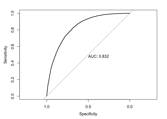
test_roc_boost = roc(diabetesTst$Diabetes ~ test_prob_boost, plot = TRUE, print.auc = TRUE)
Model comparison
metrics <- rbind(
  c(testMatrx_03$overall["Accuracy"],
    testMatrx_03$byClass["Sensitivity"],
    testMatrx_03$byClass["Specificity"]),

  c(boostMatrx$overall["Accuracy"],
    boostMatrx$byClass["Sensitivity"],
    boostMatrx$byClass["Specificity"]))

rownames(metrics) <- c("Logistic", "Boost")

metric_comparison <- as_tibble(metrics, rownames = "Model")

kable(metric_comparison)
| Model | Accuracy | Sensitivity | Specificity |
|---|---|---|---|
| Logistic | 0.7483556 | 0.7675806 | 0.7292958 |
| Boost | 0.7513968 | 0.7978406 | 0.7053521 |
Evaluate
Two methods were used to classify Diabetes, logistic regression and gradient boost. For the logistic method, models with multiple cutoffs were used to identify the most accurate one, with the 0.5 cutoff yielding the best results. The model exhibited the best trade off between Accuracy, Sensitivity, and Specificity, with the values, respectively, of 0.74, 0.76, 0.72. The model was able to identify instances of diabetes with 74 percent Accuracy, with the true positive and negative rates sitting at 76 and 72 percent, respectively. To ensure that these metrics were not the result of under or over-fitting, the test and train error were compared. With both values sitting around 0.25, there was little reason to suspect a poor fit model since the errors were close in value. That is to say that the model is able to generalize well on unseen data. The AUC value of 0.828 suggests that the logistic model performs well at discriminating between positive and negative cases. That is, the model has an 82.8% chance of correctly ranking a positive case higher than a negative one.
A gradient boost model was created using xgboost. In this model, “weak learners”, or stumps from a decision tree, are aggregated into an ensemble model. The residuals from this model are then scaled by a learning rate and fitted to a new model. This ensures error is reduced without over-fitting. The effects of the xgboost model are evident in the errors, with the train and test sitting at 0.23 and 0.24, respectively. This improvement in accuracy is reaffirmed by the performance metrics, with the boost model leading its logistic counterpart in accuracy and sensitivity, but shrinking 2 percent in specificity. In this case, we will not weigh specificity as heavily since our main concern is in detecting positive cases of diabetes. With that said, the boost model’s AUC of 0.832 is a slight improvement from its predecessor, indicating that it is able to distinguish between positive and negative cases more efficiently.
Conclusion
The two models above predict diabetes at an acceptable level. Both deliver solid performance metrics, with AUCs above 0.8, and both are able to generalize well on unseen data. This is true in that the train and test errors for both models are close in value. However, if one model were to be selected for classifying diabetes, we would select the gradient boost model.
The boost model led its logistic counterpart in every classification metric, and although it falters in specificity, this metric is not as important in this context. This is because the consequences of being wrongly diagnosed as diabetic is far less severe than being wrongly undiagnosed–in which case, a patient could experience diabetic ketoacidosis (DKA). This is not to say that an incorrect diagnosis is a non-issue, but for the sake of correctly identifying diabetes, a slight drop in specificity is not detrimental. With that said, the boost model is sufficient at predicting instances of diabetes at 75 percent accuracy. Moreover, the model’s ability to detect 79 percent of true cases is significant for the reasons laid out above. As such, we can conclude that the boost model is a superior option for predicting diabetes.
Work Cited
Heiser, Tom. “Prediabetes? Type 1 or Type 2 Diabetes? Making Sense of These Diagnoses.” Norton Healthcare, 18 Feb. 2025, nortonhealthcare.com/news/prediabetes-misdiagnosis/#:~:text=One%20major%20risk%20of%20this,creating%20harmful%20acids%20called%20ketones.
Kirkpatrick, Justin. “12: Applied Logistic Regression - Classification.” EC242, ec242.netlify.app/assignment/12-assignment. Accessed 7 Jan. 2025.
Teboul, Alex. “Diabetes Health Indicators Dataset.” Kaggle, 8 Nov. 2021, www.kaggle.com/datasets/alexteboul/diabetes-health-indicators-dataset.